HUBBERT’S PEAK IS HERE
Conventional oil production has now unequivocally rolled over. Unconventional production, the only source of growth in global oil supply over the last 12 years, has also significantly slowed. The only growing non-OPEC basin is the Permian in West Texas. Never before has oil supply growth been so geographically concentrated. Six counties in West Texas are now 100% responsible for all global production growth.
Conventional non-OPEC oil production peaked in 2007 at 46.2 mm b/d and now stands at 44.2 mm b/d – 4% below its peak. Including OPEC, conventional global output peaked in 2016 at 84.5 mm b/d and now stands at 81.3 m b/d – 5% below its peak. Even if OPEC has its alleged 4 mm b/d of unused production capacity (something we do not believe), conventional production would barely regain its 2016 peak.
In 2009, we tried to predict non-OPEC production growth based on every major project expected to come online over the next ten years. Based on our modeling, non-OPEC supply would begin to contract by about 200-400,000 b/d annually. New fields would not grow enough to offset underlying field depletion that we estimated at 4% in the non-OPEC world. In our 2Q18 letter, we tackled the subject again. In two essays (“Conventional Oil: The Problems No One is Talking About” and “Conventional non-OPEC Oil in Depth: Declines are Set to Rapidly Accelerate”), we discussed how conventional non-OPEC production was in terminal decline. Our research looks to have been correct.
However, the world has enjoyed a great luxury—it could ignore the problems firmly embedded in conventional oil production. Surging production from non-conventional oil sources more than offset these declines.
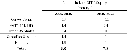
Non-OPEC oil production between 2006 and 2015 grew by 8.6 mm b/d. Conventional oil supply contracted by 1.4 mm b/d. Unconventional oil supply more than offset these declines, surging by 10 mm b/d and broken down as follows: US shales grew by 6.8 mm b/d (65% of all growth), bio-fuels grew by 1.9 mm b/d (19% of the growth), and Canadian oil sands increased 1.4 mm b/d (14% of the growth). Please note that out of this 10 mm b/d growth figure, the Permian represents only 1.4 mm b/d or 14%.
Between 2016 and 2023, unconventional production surged by another 7.4 mm b/d, representing all non-OPEC supply growth. US shales accounted for 85% of the increase. However, whereas all the major shale basins grew from 2006 to 2015, only the Permian grew after- ward. The Bakken and Eagle Ford peaked at 1.5 mm b/d in 2015, and this year are each expected only to be between 900,000 and 1 mm b/d. Significant unconventional growth also came from natural gas liquids production in the liquids-rich Marcellus and Utica, which we estimate each added 1 m b/d. This source of production growth is now set to fade, while the plateauing of the Marcellus will turn into a decline.
Between 2006 and 2015, the Permian represented only 14% of unconventional supply growth. Between 2015 and 2023, the Permian represented almost 75% of this growth.
Table 1 Change in Non-OPEC Production 2006 – 2023
 |

Source: IEA, EIA, G&R Models.
Conventional production started declining in the non-OPEC world over a decade ago. Conventional oil production has most likely turned negative in the OPEC world as well. Over the last thirty years, global oil supply growth has come from multiple geographic areas, including the North Sea, Mexico, Brazil, West Africa, and the Former Soviet Union. Over the last decade, however, these areas have had slight growth, and specific basins, such as the North Sea, have experienced considerable declines.
Consensus opinion believed global oil demand would peak in 2019 and gradually decline through this decade. Just the opposite has occurred: demand has come roaring back post-COVID. Global demand in 1Q23 surpassed 102 mm barrels per day — three million barrels above the 1Q19 (pre-COVID) level and almost 2 mm b/d above the International Energy Agency’s (IEA) 1Q23 estimate. Strong demand and faltering supply led OECD countries to release 250 mm barrels of oil from their strategic petroleum reserves to keep prices from surging. Given the seasonality in demand and China’s ongoing reopening, the 4Q23 demand could surpass 104 mm b/d.
From here on out, just six counties in West Texas must meet all global demand growth. Given the strategic importance of the Permian, it’s imperative to understand its underlying health. Using our neural network, we have updated our basin analysis, and the results are shocking. The Permian is likely less than a year from peaking and starting its decline. The only source of non-OPEC supply growth is now primarily tapped out.
After many false starts, Hubbert’s Peak is finally here.
The Permian Basin Is Depleting Faster Than We Thought
The most crucial development in global oil markets is depletion in the Permian basin. We first warned about this in 2018, predicting the Permian would peak in 2025. In retrospect, our analysis was too conservative. We now believe the basin could peak within the next twelve months. The implications will be as profound as when United States oil production peaked in 1970, starting a chain of events ultimately sending prices up five-fold over ten years. If we are correct, this could not come at a worse time for oil markets: inventories are tight, production in the rest of the world is declining, and investors are incredibly complacent.
Whenever we make long-term thematic predictions, we construct a road map of things we should expect to see. Since price is rarely a good proxy for fundamentals, we need hard data that confirms we are going down the right path, even during the inevitable periods when the oil price is moving against us. Based upon our original work back in 2018, we concluded
the Permian would roll over once operators drilled most of their best Tier 1 locations. Before peaking, per-well productivity would fall as operators drilled lower-quality inventory. This is what has happened. For the first time, productivity per lateral foot registered a 6% year-on- year decline in the Permian. According to our models, this proves the industry has drilled its best wells; basin-wide production decline is likely not far behind. With the Eagle Ford and Bakken unable to grow over the last eighteen months, once the Permian rolls over, the shale revolution will shift from growth to decline, and Hubbert’s Peak will reemerge with a vengeance.
The past decade has indeed been remarkable for global oil markets. Operators first succeeded in developing natural gas shales before adapting the techniques to the oil shales starting with the Bakken in North Dakota. The Eagle Ford was developed next, and then finally, the largest of all, the Permian, with its stacked pay potential, started its development in 2012. The results were without precedent. After having declined by 50% over forty years, the US abruptly reversed course to become the largest oil producer in the world. Shale oil production went from zero to 10 m b/d, more significant than Saudi Arabia.
The shales could not have come at a better time. In 2003, China joined the World Trade Organization, and its crude demand growth markedly accelerated. In 2005, non-OPEC production growth began to falter, forcing crude markets into a structural deficit. As inventories fell, prices rose, prompting Malthusian warnings almost daily on CNBC and Bloomberg that we were “running out of oil.”.
The shale revolution changed everything. By 2014, non-OPEC production growth reached 2.2 mm b/d, the most robust growth since at least 1966 — driven entirely by the shales.
As the shales ramped up between 2010 and 2018, they seemed limitless. However, even in the early stages of field development, there were warning signs that shale basins adhered to the same depletion principles as conventional fields. Enormous is not the same as infinite, we argued and warned that depletion would eventually take hold.
The shales seemed particularly invincible between 2014 and 2017. In the autumn of 2014, Saudi Arabia stunned the oil markets when it abandoned its role as a swing producer. Crude balances shifted into surplus in the middle of 2014, and instead of cutting production to balance the market, Saudi Arabia announced it would grow output by nearly 1 mm b/d. Immediately, crude prices fell by 15% from $75 to $60 per barrel and would drop by 65% over the next eighteen months to bottom at $26 by spring 2016. With much lower prices and capital-intensive drilling, shale developers reduced their drilling activity by 80%. In the summer of 2014, the industry turned 1,600 rigs; less than two years later, the rig count stood at only 325. Saudi Arabia relented in late 2015, with prices stabilizing a few months later, in February 2016. The shale rig count bottomed in June.
Somehow shale production stabilized and started to grow shortly after that. Even though the rig count was still down 60%, US production was again registering yearly growth as soon as April 2017. By 2018, the shales were growing by 1.8 mm year-on-year — a record, despite a rig count that remained 50% lower than in 2014.
The shales seemed to defy the laws of physics: they could grow materially despite much lower drilling activity. The industry appeared to have entered a world where it no longer needed increased drilling to boost production.
How was this possible? The answer was drilling productivity. Between 2013 and 2017, the average shale well went from averaging 70,000 barrels of oil over the first twelve months to 140,000. On the Midland side of the Permian basin, the primary source of supply growth, twelve-month productivity nearly tripled from 50,000 to 140,000 barrels.
Since each well brought on so much more oil than before, the industry could now achieve with 400 rigs, what it took 1,600 rigs to produce a few years earlier.
Conventional wisdom believed the industry had improved its drilling and completion of shale wells. The ability to stay in the zone, the choice, and the volume of proppant and fluid were all said to have resulted in sharply higher drilling productivity. Wall Street and the energy industry both promoted a consistent narrative. We felt there were several unanswered questions and undertook a study to consider what was driving surging well productivity. If the industry had radically improved drilling techniques, it would ultimately be bearish for the sector. A previous low-quality Tier 2 location could now be transformed, through enhanced drilling and completion techniques, into a top-quality Tier 1 well. As a result, the inventory of best wells would explode, and the shale basins would continue to thrive for years to come.
Modeling well performance is hugely complex. Shale basins are highly nonlinear with high degrees of variable inter-dependence. As a result, traditional statistical techniques, such as the linear regressions used by most analysts, fall short. We turned to advanced methods, including machine learning and neural networks, and achieved surprising results. Instead of improved drilling techniques, we concluded that two-thirds of the improved productivity between 2013-2018 came from favoring the best drilling locations. In 2013, 22% of Midland wells were Tier 1. By 2018, Tier 1 represented 50% of all wells. Since a Tier 1 well is nearly twice as productive as a Tier 2 well, the migration from lower to higher quality areas drove a massive amount of the improved well productivity.
The industry was not turning Tier 2 into Tier 1 but, instead, was aggressively depleting its inventory of top-quality wells.
We determined that the pace of high-grading could not continue, particularly in the Eagle Ford and Bakken. Our models suggested that by 2018, 60% of the best acreage in those two earliest developed basins had already been developed. The Permian was developed last, so it still had over 60% of its Tier 1 areas left to drill, but we were concerned that given its pace, it too could soon become depleted. In our 2Q2019 letter, we predicted the Eagle Ford and Bakken would quickly peak while the Permian plateau in the late 2020s at 6.5 m b/d. While the Permian would still manage to grow another 2.5 m b/d from 2018 levels, its annual growth rate would slow materially from 500,000 m b/d per year between 2013-2018 to only 200,000 b/d between 2019 and 2029.
The impacts of COVID-19 complicated our models; however, our predictions have been directionally sound. All three basins declined sharply in 2020, as fears of breaching inventory capacity forced prices negative and led to widespread shut-ins of existing wells. Between March and May 2020, total production from the Eagle Ford, Bakken, and Permian fell by over 2 m b/d. Since then, all three basins have brought back their shut-in production, but in the case of the Eagle Ford and Bakken, production remains 500,000 b/d below the pre-COVID March 2020 highs. Neither play has grown since November 2020. Just as our models indicated, the Permian was the only basin still able to grow. Between March 2020 and May 2023, the Permian rose by 800,000 b/d to an all-time high of 5.7 m b/d.
Unfortunately for global oil markets, our models tell us the Permian is also very close to plateauing. If we are correct, then the only source of non-OPEC growth over the past 15 years is about to shift from growth to decline.
We have spent the last several months completing and updating our machine-learning models. We owe a debt of gratitude to both the data and analytical insights provided by NoviLabs (formerly ShaleProfile), our data providers. Since we first built our neural network in 2018, NoviLabs has dramatically enhanced its database. Whereas our original models relied upon geographical data (i.e., where a company drilled a well) and completion data (i.e., how a well was drilled and completed), our latest model incorporates actual subsurface geological data. Our original models inferred the best Tier 1 acreage based on nearby well results. Our new model adds geological parameters such as thickness, thermal maturity, organic content, oil in place, porosity, and permeability to make accurate well-quality predictions. We have also been able to more accurately attribute well-quality changes to each parameter using state-of-the-art SHAP values. While a complete discussion of SHAP values is beyond the scope of this letter, in summary, they explain how a change in inputs impacts well quality in a very interpretable manner.
Between 2013 and 2018, Permian productivity increased by 153%, with three-quarters of the increase explained by improved geology—moving the drilling rig from a tier 2 to a tier 1 location–and increased lateral lengths. When we wrote in 2019, we predicted that Permian per-well productivity was likely nearing its maximum, and, in retrospect, that was correct. Between 2018 and 2021, per-well productivity growth slowed dramatically, advancing by only 20%, all of which was due to longer lateral lengths. On a per-lateral foot basis, there was no growth at all.
The Wall Street Journal recently wrote a pivotal article (using data from NoviLabs) stating that Permian per-well productivity fell in 2022 for the first time in the field’s shale development history. Our analysis confirms these results: Permian per-well productivity fell 8% last year. The drivers of the lost productivity will only get worse. Our models tell us geological depletion will continue. Permian produces are now being forced to drill worse quality rock for the first time.
Furthermore, the Permian is also suffering from parent-child setbacks. In the early days of shale development, producers would often drill a single horizontal well to test different parts of the basin and satisfy lease obligations that often require drilling a well within an allotted period. Later, the developer returns to the best areas and drills several more wells from a single pad to develop the resource economically. Producers now realize that the so-called “child” wells produce between 5 and 20% less oil than expected. In 2012 we estimate that only 30% of wells drilled in the three significant shale basins were “children.” By 2022, that figure had reached 85%. In Tier 1 areas, effectively, all current wells are children, with lower-than-expected productivity.
After several years of aggressive high-grading, we estimate the Permian has now developed nearly 60% of its Tier 1 acreage. The Eagle Ford and Bakken hit this same level of Tier 1 development in 2018, right before production stopped growing. Today, the Bakken is the most developed of all three major basins, with 66% of its Tier 1 wells developed and nearly 90% of its best areas thoroughly drilled. When we first made these predictions in 2019, we expected the Permian had until 2025 before it reached these levels, but in retrospect, we were likely too optimistic.
King Hubbert hypothesized that a hydrocarbon basin would peak once half the recoverable reserves were produced. Even though his theories referred to conventional basins, we have long believed that shale basins should behave similarly. The difficult task is estimating the recoverable reserves from each basin. Luckily, our models can help here as well. We count 7 and 9 billion barrels of recoverable oil in the Eagle Ford and Bakken, respectively, of which 65% and 55% have been produced. Consistent with Hubbert’s theories, both basins have been unable to grow after crossing the 50% mark. The Eagle Ford produced half its recoverable reserves in August 2019; production has fallen 18% since. The Bakken produced half of its reserves in 2022, and production has since been flat. Our models tell us the Permian will ultimately recover 34 bn barrels of oil, of which 14 bn or 41% have already been produced. At current production levels, the Permian will have produced half its recoverable reserves sometime in late 2024; at this point, it will most likely stop growing, just like the other two basins.
Predicting a peak in basin-wide production is difficult; fields can often eke out slightly more growth than initially anticipated. Whether the Permian peaks next month or nine months from now is subject to more variability than any analyst can confidently predict. However, we know that geological depletion is clearly taking place and will likely get worse. Year-on-year growth in the Permian appears to have peaked at 656,000 b/d in February and is already down to 480,000 b/d year-on-year in May. While the data may be lumpy, we expect this slowdown to continue and believe we may not see any year-on-year growth by the end of next year.
Finding attractive investment opportunities in shale E&P companies will become very difficult. Here too, we believe our machine-learning models can help. Based on current drilling activity, the average publicly traded Permian company will run out of Tier 1 drilling locations within 3.7 years. Our core positions, on the other hand, likely have between five and ten years of high-quality drilling ahead of them. As productivity becomes harder to achieve, these companies should present good opportunities. Already, we have seen rumors of Exxon Mobil (XOM) seeking to acquire Pioneer Natural Resources. We own Pioneer and do not know whether these rumors are true. However, we firmly believe that as the market realizes how little Tier 1 acreage remains, those with the best inventory will be treated as valuable assets.
If we are correct, the age of shale growth is now behind us, and the reality of Hubbert’s Peak is at hand. The immense growth of the shales over the past decade has blinded many analysts to the declining trends in global conventional production. That luxury is about to end.
The US Reserve Currency & Commodities
In 2016, we published the following chart comparing commodities to the Dow Jones Industrial Average. Mr. Gundlach of DoubleLine had issued a similar chart; however, his version only went back to the inception of the Goldman Sachs Commodity Index in 1970. We were interested in studying previous cycles and decided to construct our equivalent index back to 1900.
Incredibly, by 2016 commodity prices had sold off to such an extent that they were the most radically undervalued in 120 years. The only times that came close were in 1929, 1969, and 1999. Following every prior period of radical undervaluation, commodity and natural-resource related investments dramatically outperformed, both in absolute and relative terms. This cycle, we argued, should be no different. While the 1970s and 2000s bull markets are well studied, we were stunned that commodities and natural resource equities did well during the Great Depression. A simple equally weighted portfolio of energy, base metal, precious metal, and agricultural stocks bought at the market peak in 1929 more than doubled by 1938 compared with the broad market that remained 50% lower. Indeed, owning commodity stocks throughout the Great Depression was the only way to preserve one’s wealth. Given the concerns of an impending recession, those worried about resource investing should take note. During the 1970s, a similar portfolio split evenly between the four sectors advanced by 500%. While the S&P 500 managed to advance by 170%, it barely kept up with inflation. Investing in natural resource equities was one of the few ways to grow purchasing power. From 1999 to 2010, there were two massive market pullbacks (the dot com bubble and the Global Financial Crisis) and the most significant financial crisis since the Great Depression. While the S&P 500 was flat between 1999 and 2010, with great turmoil, a similar portfolio of resource equities surged by 300%. Again, resource stocks were one of the few days to avoid the calamities of the early 2000s.
The more we studied the three periods of radical commodity undervaluation, the more we recognized certain similarities.
First, for commodities to become radically undervalued relative to stocks, they must decline in price. Before every extreme low in our analysis, commodity prices fell sharply. Following the end of World War I, there was a strong and sustained bear market in commodities through the 1920s, during which most prices fell by 60%. There was a drawn-out commodity selloff from 1945-1960 that saw prices fall by 20%. Commodity prices were weak once again throughout the 1980s and 1990s. Gold peaked in 1980 at $850 per ounce and spent the next two decades falling by 70%. Crude peaked at $45 per barrel] in 1979 and lost 75% over the next eighteen years before bottoming at $11 per barrel in 1999. The recent commodity bear market was the most severe in many regards. After peaking at $145 per barrel in the summer of 2008, crude prices spent the next 12 years falling more than 100% to reach the unfathomable price of -$45 per barrel.
Second, excess money creation and easy credit preceded every period of radical commodity undervaluation. In the 1920s, the US Federal Reserve engaged in its first bout of quantitative easing. Britain had suspended gold convertibility of the pound during World War I. Once hostilities ended, Britain was desperate to return to the gold standard at its pre-war exchange rate. Federal Reserve Chairman Benjamin Strong tried to help Britain achieve its goal by lowering short-term US interest rates despite a robust US economy, helping devalue the dollar and push the pound. Strong bought significant quantities of short-term treasury bills in 1924 and 1927.
Throughout the 1960s, the combination of Johnson’s Great Society programs and Vietnam War spending necessitated the help of an accommodating, albeit reluctant, Federal Reserve. Multiple banking, financial, and currency crises, requiring several rounds of accommodative monetary policy, bedeviled the 1990s. Most recently, the lowest interest rates and loosest monetary conditions in human history characterized the 2010s. The Federal Reserve’s balance sheets exploded from $900 bn in 2007 to $8 tr by 2020. By the summer of 2020, over $17 tr of global bonds sported negative nominal interest rates – a first in four thousand years of human history.
Third, each period of radical commodity undervaluation was associated with an investment mania elsewhere in the market. This observation follows logically from the last. Loose credit and excessive money printing lead to speculative malinvestment and asset bubbles. The 1920s saw a massive stock market boom culminating with the famous “Coup de Whiskey,” administered to the market when Strong injected ample liquidity into an already robust economy. Technology stocks did remarkably well. Shares of Radio Corporation of America were market leaders, with rampant speculation fueled by unprecedented use of financial leverage. A stock market crash and the most significant bear market in US history followed the blow-off top in the fall of 1929. The 1960s and early 1970s saw substantial bull markets accompanied by intense stock market speculation in new areas, such as conglomerates and growth stocks. The result was the “Nifty Fifty, in which fifty stocks, each with a P/E ratio 50x, could do no wrong. Driven by easy money and the internet introduction, the US market reached its greatest over-valuation by the late 1990s. The past decade has had several asset bubbles and investment manias. FAANG stocks, cryptocurrencies, and passive index funds all contribute to the “everything bubble” of the 2010s.
After studying these trends for several years, we concluded that the commodity capital cycle intimately connected them. Edward Chancellor’s “Capital Cycles” proved invaluable in helping us refine our views. An idealized commodity capital cycle progresses as follows: commodity prices are high, and producers enjoy a period of super-normal profits. Capital flows in chasing returns and results in elevated producer valuations. Companies raise vast amounts of money and deploy it on new projects. Supply increases and overshoots demand, pushing the market into surplus and depressing prices. Projects, underwritten at much higher commodity prices, become impaired and large amounts of capital are written off. Investors begin to turn away from commodity investments, and money pours out of the space, depressing valuations and leaving companies unable to tap capital markets. Investment stops, and companies abandon new projects, grinding supply growth to a halt. Depletion inevitably takes hold, tightening the market until eventually, surplus gives way to deficit, and a new cycle begins.
This framework perfectly explains the periods of radical commodity undervaluation we studied above. A commodity boom that saw production grow sharply preceded each period. Supply overwhelmed demand, pushing down prices. Investors left the industry for dead and moved into the investment mania of the day. Cheap credit allowed for malinvestment, pushing the mania further and making commodity investments even less appealing. Commodity producers became capital-starved, and depletion took hold.
The remaining question is what ended each period of radical commodity undervaluation and ushered in the new bull market. The answer is a fundamental shift in the global monetary system. By 1929 it was clear that Britain would be unable to keep the Pound tied to gold, effectively ending the classical gold standard in place since the early nineteenth century. The resulting financial turmoil included US history’s most significant stock market crash and a global banking crisis. Eventually, the unrest forced a massive 60% devaluation of the US dollar in 1934. The bottom in commodities relative to financial assets occurred concurrently with the ending of the classical gold standard.
During the 1960s, the United States ran ongoing budget deficits to fund the combination of Johnson’s Great Society program and the Vietnam War. As a result, starting in the mid-1960s, the Treasury suffered persistent outflows of gold as foreign governments exchanged their excess dollars for gold bars, per the 1944 Bretton Woods Exchange Agreement. By 1967, gold outflows had grown so large that the Treasury risked no longer being able to honor its commitment to back each dollar with 25 cents of gold. In 1968, Johnson signed into law a bill eliminating the dollar’s gold backing. While most believe Nixon took the dollar off gold, it was Johnson who stopped the dollar’s required gold backing. It took three years to eventually deplete the Treasury’s gold holdings to the point where Nixon no longer allowed convertibility in 1971. Although it received little attention then, this shift in monetary policy in 1968 corresponded with the beginning of the enormous commodity bull market that would last the next thirteen years. The resulting colossal dollar depreciation was again a significant stimulant to the massive commodity bull market that raged throughout the 1970s.
The monetary shift that precipitated the end of the 1999 commodity bear market is less noticeable but equally important. Throughout the 1990s, many emerging markets chose to peg their currency to the US dollar. The rationale was that the Treasury would provide emergency liquidity via US dollar swap lines in a financial panic. The collapse of Long Term Capital Management in 1998 led to an emerging market rout that escalated once it was clear the Federal Reserve would not bail out emerging markets. Several currencies collapsed overnight. Between 1997-1998 the Indonesian rupiah, Thai baht, Malaysian ringgit, and South Korean won tumbled between 50 and 85%. Following the crisis, many emerging market economies instead adopted a managed currency policy in which they would suppress the value of their currency to promote exports.
Undervalued currencies resulted in surging current account surpluses, the proceeds of which were recycled primarily into US Treasuries. In 1996, Asian economies ran net current account deficits totaling 2% of GDP. By 2005 these same countries ran current account surpluses totaling 5% of GDP. These surpluses resulted in trillions worth of US dollar accumulations which were recycled back into Treasuries. The new monetary system, born of the 1998 currency crisis, enabled OECD countries to borrow and overconsume for almost a decade, resulting in the 2008 housing and related global financial panic. Emerging market currency suppression again massively stimulated commodity consumption in the emerging world— with China being the best example.
As we enter what we believe to be a decade-long resource bull market, three of the four pre-conditions are unequivocally in place. Since 2010, commodity prices have pulled back more than 70%. The bear market severely impacted cash generation in many commodity industries. Companies have slashed capital spending dramatically. Money creation reached extremes in the 2010s. In the summer of 2008, the US Federal Reserve’s monetary base was
$850 bn, or approximately 6% of GDP. By the end of 2021, it had exploded to almost $6.5 trillion representing an incredible 30% of GDP. The money creation over the last twelve years has no parallel in US history, exceeding those in the 1920s, 1960s, and 1990s. Easy credit has led to an “everything” bubble. Equity valuations are nearly as high as in 1999, while at the peak, over $17 tr of fixed-income securities sported negative nominal yields – a first in history. FAANG stocks and crypto-currencies are the mania of the day, much like RCA was in the 1920s, the Nifty Fifty were in the 1960s, and dot-com stocks were in the 1990s.
The only missing element has been a shift in the global monetary system. The final piece may be coming into place: the US dollar might be on the verge of losing its reserve currency status. A change in the dollar’s reserve currency status would be the most impactful market shock of the last forty years. According to our analysis, it would also most likely correspond with a period of robust commodity performance. The monetary regime changes in 1930, 1968, and 1998 were hugely stimulative for commodity prices, and we believe the monetary regime change that will take place this decade will be no different.
Following the Bretton Woods Agreement in 1944, the US has enjoyed a unique advantage: nearly 90% of global trade has been settled in US dollars. When Australia sells coal to China, they pay in dollars. The result has been a persistent demand for dollars outside the US to facilitate global trade settlement. US dollars are recycled into Treasuries, allowing the US to run persistent deficits. Critics have called the current system unsustainable for years and warned that a change is near.
Luke Gorman of Forest For The Treeshas written about the end of the US dollar reserve status for nearly a decade. We were never convinced a change was imminent, given we saw no actual evidence countries were moving away from the dollar. While the arguments made sense, China continued buying Australian coal in dollars, and foreign Central Bank Treasury holdings remained elevated. The US reserve currency status may have been unsustainable, but at the time, it appeared intact.
We believe this is starting to change. The past twelve months have seen a spate of announcements of countries looking to settle trade in currencies other than the dollar. Although details remain scarce, Saudi Arabia has discussed settling its oil sales in renminbi. All sanctioned Russian oil sales have been paid for in renminbi to avoid the SWIFT banking system necessary for US dollar settlement. In April 2023, the Brazilian government announced intentions to set up the infrastructure to settle trade in renminbi. In the strongest rebuke of the current US dollar reserve currency system, Brazilian President Lula rhetorically asked before a group in China: “[…] why all countries have to base their trade on the dollar. Why can’t we do trade based on our currencies? […] Who decided that the dollar was the currency after the disappearance of the gold standard?” Even in Europe, the sentiment appears to be changing: TotalEnergies (TTE) agreed to sell LNG into China and settled in renminbi.
Zoltan Poszar, Louis Gave, and Luke Gorman have written some of the best research on the changes now affecting the global monetary order. Some analysts believe fifteen years of excess money printing is to blame, while others cite the “weaponization” of the dollar or the ongoing political dysfunction in Washington.
To some extent, the causes are unimportant. What matters is that the move away from the dollar has started. If this trend continues, it would represent the end of the US dollar as the global reserve currency. The writing has been on the wall for a long time, but the change is only occurring now. That is what matters.
Every other period of commodity undervaluation culminated with a shift in global monetary regimes. This time will likely not be different. Proponents of the US dollar argue that no other currency can meet the requirements of a reserve currency. While much talk has centered on the renminbi, China maintains a mostly closed capital account — a clear impediment to a reserve currency.
As commodity exporters amass renminbi, there is no apparent outlet for them to convert their capital. Of course, Chinese goods remain a strong export market; however, these are not enough to balance the trade with commodity producers. While Louis Gave correctly points out that China is building a robust Chinese Government Bond market, this only pushes the problem into the future when the bonds mature. Indeed, commerce covets the US dollar because it is a unit of exchange accepted as collateral worldwide. CGBs do not hold the same appeal.
Any move by China to displace the US dollar as a reserve currency must include some degree of gold convertibility. Foreign holders could then convert some portion of their trade surplus from renminbi into gold via the Shanghai gold exchange. China has accumulated vast amounts of gold in recent quarters, making such an outcome more plausible. If this were to happen in earnest, commodities would go from radically undervalued to radically overvalued — likely led by gold. Every other commodity bear market ended with a shift in the global monetary system and a devaluation in the dollar that stimulated resources. The implications will be profound for many asset classes. However, history suggests the biggest beneficiaries will be commodities and their various producers. Investors must be aware and seek to protect themselves.
1Q23 Market Commentary
Two additional Fed rate hikes, and strong rhetoric about more to come, put downward
pressure on most commodity prices in the first quarter as investors became convinced 2023 would see a material economic recession. Only two commodities displayed any strength: gold and copper. Everything else was flat to down.
With its heavy energy exposure, the Goldman Sachs Commodity Index fell almost 6%. The Rogers International Commodity Index, which has much higher exposure to metals and agricultural commodities, fell nearly 5%.
Natural resource-related stocks were mixed. The S&P North American Natural Resource Stock Index (IGE) fell 2.9%, while the S&P Global Natural Resource Index (GNR), which has a much higher weighting to metals and agricultural-related equities, rose 0.1%. Equity markets overall were buoyant in the first quarter. The S&P 500 stock index and the MSCI All-World Index rose 7%.
Natural gas led the commodity markets lower during the quarter. A warm North American winter and an exceptionally warm European winter flipped both markets from deficits to surplus. In the US, winter was 2.7 degrees F warmer than normal, ranking it the seventeenth warmest on record. The average winter temperature in Europe averaged almost 3 degrees F above normal, placing the 2022-2023 winter as the second warmest on record.
The mild weather resulted in very low heating demand, which depressed US natural gas prices by 50% during the quarter. Prices in Europe fell by 36%, while Asian LNG fell by 55%. Longer-term weather trends are impossible to predict. Investors should use unexpected weather conditions pushing gas markets to extremes as selling or buying opportunities.
As we discuss in the natural gas section of this letter, the vast pullback in North American natural gas prices has presented investors with a tremendous buying opportunity. The trends first outlined in our 1Q22 essay, “The Gas Crisis is Coming to America,” are still all in place; the exceptionally warm weather has simply pushed them out. Even with warm weather, 100% of the storage surplus occurring over the last eight months can be attributed to the fire at the Freeport LNG facility in June last year, which took offline two bcf/d of export capacity. Freeport is again operational, and with the Marcellus gas fields plateauing and six bcf of additional LNG capacity coming on stream in 2024, we believe North American natural gas convergence with international prices could happen much faster than anyone expects. The weather has presented natural gas investors with a tremendous buying opportunity, and we recommend investors use it to their advantage.
North American and international coal prices followed natural gas down as traders worried about natural gas-to-coal switching in the United States and Europe. Illinois Basin coal fell by almost 60%, and Central Appalachian coal fell by 45%. Eastern US coal prices had a huge run in 2022 as European natural gas prices nearly hit $100 per MMBtu in late August. Traders
bid up any high-BTU coal that could be exported to Europe, and now these same coals are pulling back in sympathy with European natural gas prices. International thermal coal also pulled back during the first quarter. Richard’s Bay South African coal pulled back 30%, while Newcastle Australian fell 55%. Given its “pariah” status, no industry has been more capital-starved than coal over the last ten years. As the structural deficit in global natural gas comes to the fore, coal prices should again become price leaders as this decade progresses. We have just started an enormous commodity bull market, similar to the commodity bull markets of 1929-1941, 1968-1980, and 1999-2011. In each of those bull markets, coal equities were the best-performing sector from trough to peak. Given underlying fundamentals, depressed valuations, and a complete lack of institutional interest, we believe coal equities could again become the best-performing equity group when this bull market is over.
Oil prices were weak on recessionary fears. West Texas Intermediate (WTI) and Brent prices fell almost 6%. Oil-related equities also displayed a downward bias. The S&P E&P index (XOP) fell nearly 6%, while the VanEck Oil Service ETF (OIH) fell almost 9%. Because of Fed-induced recessionary fears, bearish psychology continues to buffet oil markets. Investors worry that demand will be severely impacted as we progress through 2023. Although we did see some weakness in oil demand from November 2022 to January 2023, most of this weakness is likely attributed to the hot Northern Hemisphere winter. As we enter spring, weak demand has reversed, and global inventories have resumed moving lower. All our indicators show global demand remains significantly above consensus. In the opening section of this letter, we detailed our view that oil supply growth will end sooner than any analysts realize. We are almost 100% dependent on the Permian basin for any supply growth, and the basin shows signs of depletion. Permian production could peak entirely sometime in the next twelve months. Disappointing supply, strong demand, falling inventories, and bearish psychology could result in attractive returns over the next 12 months for those willing to ignore the consensus.
Copper was the only commodity apart from gold that advanced in the first quarter, rising by 7.5%. Other base metals were mixed: nickel fell 20% (giving back their 4Q22 gains), lead fell 8%, zinc fell 2%, and aluminum prices increased 1%. Base metals equities were strong during the quarter. The S&P/TSX Global Base Metals ETF (XBM CN) rose 8%, while the COPX rose 9%.
Short-term fundamentals in global copper continue to strengthen. Last year was another in which copper demand growth significantly outpaced mine supply growth. According to the World Bureau of Metals Statistics (WBMS) 2022, copper demand rose a very robust 3.8%, while mine supply grew by less than 1%. Data for the first two months of 2023 suggests Chinese demand is surging as COVID-19 restrictions were lifted. According to WBMS, Chinese consumption advanced an incredible 18% for the first two months of the year compared with the same period in 2022. Many analysts finally agree that the copper market has become a long-term structural deficit. Depletion continues to drive supply disappointments, despite the contribution of large new projects such as Ivanhoe Mine’s world-class Kamoa-Kakula in the Congo.
Copper remains our favorite base metal; however, we are becoming uncomfortable with how many analysts and consultants have turned wildly bullish. Now that everyone seems to agree on copper, are we setting ourselves up for disappointment? We remain copper bulls, but our copper section will explore where we could be wrong in the coming decade.
Agricultural markets corrected in the first quarter. Corn, soybeans, and wheat fell 3%, 1%, and 13%, respectively. Fertilizer prices often pull back ahead of the planting season, and this year was no different. Urea declined 30%, while phosphate and potash each fell 20%. Agricultural commodities peaked in 2Q22; since then, corn has fallen 20%, soybeans are down 15%, and wheat has fallen by half. Despite these moves, grain prices remain significantly higher than their pre-COVID levels. Corn is 80% higher than it averaged in 2019, soybeans are 70% higher, and wheat is up 50%.
Fertilizer prices followed a similar pattern. Urea, the solid form of nitrogen, is now off 60% from the post-Russian invasion highs, while potash is off 55% and phosphate is down 40%. However, even after these pullbacks, fertilizers remain 50-100% above their 2019 averages. The first quarter is always quiet in terms of agricultural data. The only significant development was the initial USDA prediction of planting intentions for corn and soybeans, released on March 31st. Farmers are expected to plant 4% more corn, while wheat plantings are expected to be 8% higher than last year.
The market’s focus will now turn to the weather. As discussed in our 4Q22 letter, large sections of the western and central corn belts are experiencing severe drought. Above-average precipitation across large sections of Ohio, Indiana, Illinois, and Wisconsin has alleviated some of the worst-hit areas; however, large swaths of the central and western corn belts remain under severe drought. Western Canada, a significant growing region, suffers from extreme drought conditions. As a result, prices will likely be very weather sensitive through the growing season, especially if dry patterns develop during the summer months.
Gold and its related equities provided a rare pocket of strength during the quarter. Gold rose almost 8%, while gold stocks (as measured by the GDX) rose 13%. Other precious metals were flat to down. Silver and silver stocks (as measured by the SIL) were up less than 1%. Reflecting their greater economic sensitivity, platinum, and palladium fell 7.3% and 18%, respectively. In our last letter, we recommended investors significantly increase their gold exposure. Gold never reached the oversold condition seen back in the fall of 2018. However, factors such as extreme central bank buying and accumulation by Western speculators are likely signaling the corrective phase in precious metals, which began in the summer of 2020, is coming to an end. Since we wrote, gold has risen sharply and almost broke through the all-time high of $2,050 set in August 2020. We believe the next leg of the gold bull market has begun. Investors need to own gold this coming decade to maintain wealth and purchasing power and act as a significant source of profit.
Uranium prices advanced quietly during the quarter. Uranium prices started the year at $48 per pound and, by quarter’s end, had crept above $50. Despite the rally in a very challenging resources market, we have noticed that many investors are incredibly bearish. As a barometer of investor sentiment, we track (and own) the Sprott Physical Uranium Trust (OTCPK:SRUUF), a closed-end fund that holds physical uranium. When investors are bullish on uranium, the Sprott Uranium Trust often trades at a significant premium to the value of its uranium holdings. At its peak in September 2021, it traded at a 30% premium to NAV. In contrast, when investors turn bearish, the Sprott Uranium Trust can trade at a discount to NAV. After starting the year at a slight premium, the Trust has sold at an ever-larger discount to NAV. Currently, the Trust trades at a 14% discount to NAV – the steepest since the broad market selloff experienced in the summer of 2022. When the Trust trades at a premium to NAV, it can issue new shares and purchase uranium. When it trades at a discount, this option is not available (although it should be noted that, unlike the GLD, the Trust never has to sell uranium to redeem shares). We believe the absence of Sprott in the market explains why 1Q23 was so quiet for uranium markets.
Financial players will be a huge force in global uranium markets, and the Sprott Physical Uranium Trust will become their preferred speculative vehicle. Our models tell us the physical uranium market is now in deficit and that quickly mobilized spot volumes are becoming scarce. Over the past several years, stockpiled materials from the ongoing closure of Japanese reactors post-Fukushima made sourcing uranium easy, but these stockpiles are now worked off. The next upward move in uranium could be particularly strong and chaotic. Speculators will eventually realize they can bull the Sprott Physical Uranium Trust, force a premium, have the Trust issue shares, and permanently sequester physical material. Although this strategy would not work in a well-supplied market, it could create sharp price increases when physical material is scarce as utilities are forced to compete with speculators for volumes. Uranium is bullish on its own; however, this unique dynamic could cause prices to surge.
Central banks are key to understanding the difference between the 1970s and today
We are using the 1970s as an analog for precious metals this decade. So far, it is proving to be prescient. By 1974, silver had significantly lagged gold for two years and staged a furious catch-up rally. From late 1973 to 1Q74, silver surged 125%. Incidentally, this “catch-up” rally marked the end of the first leg of the great bull market of the 1970s. Over the next two years, gold and silver both fell 45%, while gold stocks collapsed 70%.
We believe the current bull market started in 2018 when gold hit $1160. Silver lagged gold for two years, as it did in the early 1970s, before staging a similar catch-up rally in the summer of 2020. Over the next four months, silver would surge nearly 150%. Just like in 1974, silver’s catch-up was a sign the first leg of the bull move had ended.
In 1974, silver’s correction lasted two years, bottoming in 1Q76. Gold bottomed six months later in August. Silver’s correction lasted two years, bottoming in August 2022, with gold bottoming three months later in November. We are at the equivalent of 1976; the next leg of the bull market is underway.
Interest rate activity was similar in the two periods as well. The Federal Reserve aggressively raised interest rates in the summer of 1973, before the Arab oil embargo. From early 1973 until mid-1974, short-term rates doubled from 7 to 14%. Inflation peaked shortly after at 12% when real rates were positive by 2%. This time, the Federal Reserve raised its funding rate from zero to 5% in a year, and according to the latest inflation data, real rates are again slightly positive.
One noticeable difference between the two periods: the current selloff was much less severe than in the 1970s, despite both periods experiencing material rate increases. In 1974, gold and silver fell 45% while the stocks fell 70%. This time, gold only pulled back 20%. Silver fell 40%, and the stocks “only” fell 50%. Both precious metals and the associated stocks have also rebounded much faster compared with the 1970s.
Gold and silver stocks are only 15% away from their 2020 peaks, while gold is close to a new all-time high. By comparison, silver took six years to surpass its 1974 high, while the stocks took four years. Despite the surge in short-term interest rates, the correction has turned out to be much less severe than in the 1970s.
We believe central banks explain the difference. Our 3Q20 letter highlighted how central banks had stopped buying gold. Between 2019 and 2020, central bank purchases fell from 630 to only 273 tonnes. We warned that gold would remain under pressure if this behavior persisted. In retrospect, we worried needlessly. By 2021, central bank purchases rebounded sharply to 460 tonnes, and by 2022, they surged to 1,140 tonnes – by far the most significant amount over the last seventy years.
Central banks continue to buy aggressively. For the first two months of 2023, central banks purchased over 228 tonnes of gold, an annualized rate of 1,400 tonnes.
China remains the dominant buyer. They purchased twenty-five and eighteen tonnes in February and March, respectively, making it five consecutive months of purchases. China added 120 tonnes, bringing their total reserves to over 2,000 tonnes. While Chinese buying has been prodigious, it still represents less than 4% of total reserves. Singapore purchased forty-five tonnes in January, increasing its holdings by 30% in its largest transaction since 1968. India reentered the market, purchasing seven tonnes in the first quarter compared with seventy-seven and thirty-tree tonnes in 2021 and 2022, respectively.
As we wrote in our essay, “The Coming Change in Monetary Regimes,” a new monetary system will likely emerge this decade. Under this new system, countries will use gold to balance trade differences. For example, everyone paid attention when Brazil announced it would seek to settle agricultural and iron ore trade with China in renminbi instead of dollars. They paid much less attention when Brazil doubled its gold holdings in 2021. Are the two events related? If Brazil holds excess renminbi, will they look to swap the currency for gold, completely bypassing China’s closed capital account? We believe central banks are preparing for a monetary system where they will settle trade imbalances at least partially using gold instead of dollars. This would be explosively bullish for gold. Prodigious money printing has led to current account imbalances that vastly surpass the value of the world’s gold stock.
In response to rising interest rates, western speculators shed large amounts of gold over the last two and half years. The eighteen physical gold ETFs we track shed 520 tonnes since late 2020, while speculators have also liquidated substantial paper gold on the COMEX. Since peaking in early 2020, COMEX gold traders have liquidated 350,000 contracts, representing over 100 tonnes of gold. Central bank buying has more than offset the liquidation, explaining why the pullback has been so shallow and the rebound so quick.
Interestingly, the lack of central bank silver buying explains its ongoing underperformance compared with gold. Peak to trough silver fell almost 40%, rivaling the 1974-1976 drop, and still sits nearly 15% below its 2020 peak. For the corrective phase to last, speculative liquidation must exceed central bank buying. In the previous two and half years, gold speculators liquidated 450 tonnes of gold, yet the price remains near an all-time high. Western speculators have significantly slowed their gold liquidations and are ready to enter a new phase of physical gold accumulation.
Western investors will quickly come into completion with central bank buyers, resulting in a sharp rally. Shedding in the physical silver ETFs is also slowing.
Turning to the positioning of COMEX traders, back in February, they came close to flashing another silver buy signal: speculators went 14,000 contracts net short, and commercials missed going net long by a mere 5,000 contracts. This would have been the second buy signal in the past nine months.
In mid-2018, COMEX traders accurately predicted the upward move in silver to come. We believe, once again, the COMEX is signaling a rapidly approaching sharp upward movement in silver. COMEX gold traders refuse to flash a similar buy signal. In most precious metals bottoms, both gold and silver traders simultaneously flash buy signals (most recently in 2018), and we have been pondering this divergence. The answer, again, is central banks.
Central bank buying has been so strong it has altered the trading patterns of silver and gold traders. Given the lack of any central bank silver buying, net selling pressure in response to raising rates has become far more intense than with gold, where the central banks are buying. The added selling pressure has turned the silver speculators even more bearish.
By comparison, gold net selling pressure has been much milder. Central bank buying absorbed most speculative selling. COMEX traders have positioned themselves accordingly. The result is clear: silver traders flashed two buy signals in the last six months, while gold traders flashed none. In past letters, we wrote how COMEX gold traders would provide a buy signal, especially after a sharp pullback. Given the continued strength in central bank buying, we may not get a COMEX speculative buy signal this cycle.
The corrective phase might still drag on as the Fed raises rates; however, we are getting close to the next leg of the bull market. If the 1970s analogy holds, the next leg will be explosive.
Copper: A Case Study in Contrarian Investing
“There isn’t enough copper in the world—and the shortage could last till 2030,”
Wood Mackenzie on CBNC Feb.6, 2023
“World copper deficit could hit record; demand seen doubling by 2035,” S&P Global, June 14th, 2022
“Copper Mine Flashes Warning of “Huge Crisis” for World Supply. There’s a huge crisis. We cannot supply the amount of copper in the next ten years to drive the energy transition and carbon zero.” Doug Kirwin, Bloomberg May 2nd, 2023
In our 2Q2016 letter, we reported weak copper mine supply growth, anticipated the struggle to meet demand, and warned of a significant structural deficit in years to come. Underpinned by excellent research, it was an alarm investors did not heed. By 2016, copper prices had declined by 60% over the previous six years, and bearish investors had no interest in hearing a bullish story. For contrarian investors, it was the perfect time to get involved. Today, copper prices have rallied 150% off their 2016 bottom, and our investment thesis has become accepted by nearly everyone.
As investors, we prefer to be contrarian and often feel uncomfortable when everyone agrees with us. As such, is it time to give up our bullish stance on copper? We pride ourselves in researching investment opportunities when prices are depressed, investors are bearish, and trends have emerged that signal the bear market is ending and a new bull market is about to begin. The longer a bear market drags on, the more pessimistic investors become, and the more we like to roll up our sleeves and undertake large research projects that uncover newly emerging trends often missed by other investors.
We strive to complete our research (and make our investments) at least a year before The Wall Street Journal or Financial Times writes about the trends. Our work on copper from 2016 is a perfect example of our research and investment process. Copper peaked at $4.65 per pound in the first quarter 2011 and entered a grinding four-year bear market. Copper prices finally bottomed at $1.90 in the first quarter of 2016 — down a hefty 60% from the 2011 highs.
Several massive new copper projects were due to come online in 2015 and the surge in mine supply drove prices lower. Copper production grew by 4.5% in 2015 before surging by 6% in 2016. The new mines produced a bearishness last seen fifteen years prior when copper prices bottomed at 60 cents per pound.
There were reasons to be bullish for investors willing to ignore the pervasive pessimistic psychology. Not only was mine supply growth set to slow significantly, but new sources of demand were emerging that drew little attention in the investment community.
Our 2Q16 Natural Resource commentary “Renewables and Upcoming Massive Bull Market in Copper” outlined the high copper intensity needed to generate electricity from renewable sources such as wind and solar.
The diseconomies of scales associated with generating electricity from widely dispersed power units, combined with the extremely low-load factors, means that the copper intensity needed to generate electricity from renewable sources is orders of magnitude higher than from conventional sources. In fact, when adjusted for the additional capacity needed to compensate for renewable’s miserably low load factors, the copper intensity to actually produce electricity from renewable sources is estimated to be thirty to forty times greater than what is needed to generate electricity from conventional power plants.
After outlining various demand scenarios, we continued:
To put these figures in perspective, over the last fifteen years, copper demand has increased by an average of approximately 500,000 tonnes per year. Between now and 2020, we project that renewables will represent 400,000 of entirely “new” copper demand and that by 2025, this will accelerate to 500,000 per year— so renewables have the potential to nearly double annual copper demand growth.
And we summarized:
It is unclear how the world will meet this entirely new source of copper demand. Given that copper mine supply has only grown by about 400,000 tonnes per year over the last fifteen years, it is hard to imagine how the copper market can avoid shifting into a large structural deficit over the next several years.
Copper was $2.10 when we wrote our essay. Based on our supply and demand analysis, we predicted a new bull market in copper over the coming decade. As contrarians, it was an easy call to make. We had confidence in our research, and very few (if any) investors agreed with us. Since then, copper prices have indeed entered into a bull market. In the first quarter of 2022, copper rose, nearly hitting $5 per pound. Copper stocks have also provided excellent returns. Since the summer of 2016, copper stocks (as measured by the COPX ETF) returned 180% versus 120% for the S&P 500.
As contrarians, this presents a problem. Much of what we wrote about in 2016 has happened: demand has proved much more robust than expected; supply has severely disappointed, and everyone now understands how impactful renewables will be for copper demand. Everything we wrote about six years ago has become consensus opinion and accepted wisdom. Everyone, including the major consulting firms, has taken what was once a contrarian opinion, a particularly ominous sign.
As contrarians, should we maintain our bullish outlook despite most of the industry now agreeing with us? On a short-term basis, we are maintaining our stance. Chinese demand is once again accelerating sharply. The first two months of 2023 saw Chinese demand surge by almost 20%, according to WBMS data. Indian demand, meanwhile, grew by over 10%.
These two countries will remain the most important “traditional” demand sources. Meanwhile, supply continues to disappoint. Mine supply grew by only 1.2%, far behind demand growth of 3.8%, even factoring in a considerable increase in DRC production from Ivanhoe’s Kamoa-Kakula.
Quickly mobilized inventories on the COMEX, LME, and Shanghai exchanges are now at record-low levels when adjusted for days of consumption. Given strong demand and continued weak supply, we believe copper could eventually exceed double digits sometime in the next several years.
On the other hand, we are carefully monitoring several emerging trends that could signal the end of the copper bull market sometime later this decade. On the demand side, we believe renewables could end up disappointing. We have been critical of wind and solar due to their low energy density and poor energy return on investment (EROI). We believe the multi-trillion-dollar renewable push will be the largest malinvestment in history. Europe is in the process of understanding the consequences of large-scale renewable investments. In The Wall Street Journal dated May 15th 2023, French President Emmanuel Macron suggested: “Europe may already have enough environmental regulation and doesn’t need more.” Mr. Marcon went on to call for a “regulatory break” on European environmental matters.
Perhaps President Macron has finally realized the limitations of renewable energy, both in terms of economic impact and inability to slow CO2 emissions. How long before the rest of the world comes to the same realization? As of today, the world still seems intent on going down the wrong path: the Inflation Reduction Act is a perfect example.
So long as the world remains determined to increase renewable investments, copper demand from renewables will stay positive. However, it is imperative to monitor this situation closely, especially as nuclear offers a compelling alternative. Nuclear power is highly energy efficient while producing no CO2. If renewables are a “lose-lose” proposition, nuclear power is a clear “win-win:” extremely high EROI and no carbon. Are we vastly overestimating renewable energy’s long-term impact on copper demand? We will explore the topic in an upcoming essay.
On the supply side, could we be underestimating future growth? Here, we want to discuss two potential new supply sources that few investors are discussing. First, Jetti Resources has discussed a new leaching technology enabling producers to leach low-grade sulfide ores effectively. The last major metallurgical breakthrough occurred in the mid-1980s with the introduction of SX-EW, which allowed copper producers to mine and extract copper from low-grade oxide deposits for the first time.
The industry maintained a deep inventory of such deposits but neglected them because traditional flotation technology yielded poor copper recoveries. The introduction of SX-EW enabled the producers to put these deposits into production economically. SX-EW copper went from nothing to almost 25% of world copper production by 2000. Copper was in a structural surplus for well over a decade that saw real prices fall to lows not seen since the Great Depression. Could Jetti’s technology bring about a similar surge of supply, this time from low-grade sulfide deposits? We will follow it closely, writing about it in a future letter.
Additional supply could come from introducing a new exploration tool from Ivanhoe Electric known as the “Typhoon” geophysical survey system. (For full disclosure, Goehring & Rozencwajg has a position in Ivanhoe Electric.) As opposed to the oil and gas industry, which has made considerable advancements in exploration technology over the past seventy years, the mining industry largely relies on technologies used for hundreds of years. Geologists walk along the surface with a pick hammer and a sampling “grab bag,” looking for rock outcrops and soil alterations. A geologist from the eighteenth century would feel right at home today. Given the relatively primitive techniques, it stands to reason that most significant deposits are still located reasonably near the surface. The oil and gas industry has developed exploration tools to look deep into the earth’s crust. A lack of technology restricted the mining industry to what could be found visually near-surface.
However, this might be changing as we write. Ivanhoe Electric’s “Typhoon” uses high-energy pulses and advanced neural networks to produce high-resolution images allowing exploration geologists to efficiently detect sulfide mineralization containing copper, gold, silver, and nickel deep in the earth’s crust for the first time. Ivanhoe Electric has already made one significant new deep high-grade copper discovery in Arizona using the “Typhoon” technology, and they are waiting to drill several new targets.
The industry discovered most of today’s copper mines from the surface. However, geologists agree that a considerable inventory of porphyry targets is waiting to be found at greater depths, similar to Freeport’s Serbian Timok project. For the first time, mineral geologists will now (potentially) have the exploration tools available to make these discoveries.
Oil’s Selloff Driven By SPR Releases
Inventories are essential to analyzing any commodity market, representing the intersection of supply and demand. When supply exceeds demand, inventories grow; when demand exceeds supply, they fall. By studying inventory behavior (seasonally adjusted where appropriate), an analyst can immediately assess whether a market is in surplus or deficit in near real time. Over time, there is such a strong correlation between oil prices and seasonally adjusted inventory levels that many analysts use inventory models to predict oil’s “fair value.” Presently, global and US petroleum inventories stand at 397 mm and 291 mm b below five-year averages, implying a fair price of $120 per barrel. With WTI currently trading for $70 per barrel, the discount to fair value is $50 per barrel or 45%.
What explains the difference?
As with most things, the devil lurks in the details. In this case, the question is how to treat government-controlled strategic petroleum reserves. For most of the past half-century, this distinction has been irrelevant. From 1977 (when the US first introduced its SPR in response to the first OPEC oil crisis) to 2020, US government stockpiles varied by a modest 40,000 b/d.
Everything changed when Russia invaded Ukraine. Between May and December 2022, the US depleted its strategic petroleum reserves by nearly 200 mm bbl or 720,000 b/d. Other governments followed suit, although to a much lesser magnitude. We estimate US SPR releases made up 90% of all government liquidations in 2022. To put this figure in perspective, shales grew by only 188,000 b/d in total for 2022. It is fair to say the biggest driver of oil markets last year was the change in strategic petroleum reserves.
How should investors think about such a torrent of crude oil? On the one hand, if inventories are a proxy for market balance, it makes sense to consider total global inventories. For example, if demand runs 1 mm b/d ahead of demand, total inventories would fall by the same amount. On the other hand, during liquidations, the SPR acts as a source of oil supply, no different than a new field coming online. During periods of SPR accumulation, it acts as a source of incremental demand.
Although we believe total petroleum inventories most accurately reflect actual oil balances, the market treats SPR releases as a supply source. As you can see in the chart below, the “fair value” for WTI using commercial inventories (i.e., treating SPR releases as supply) is approximately $80 per barrel – closer to the actual price.
There is a historical precedent for this distinction. Between 2001 and 2005, the US accumulated 111,000 b/d into the SPR, or 146 m b, to help insulate against production losses from the Iraq invasion. Commercial inventories declined by 3 m b over the same period. Even though total petroleum inventories grew by 140 m b on balance, WTI doubled from $30 to $60 per barrel. Investors were less concerned with total inventories, instead treating the SPR as a new source of incremental demand. Crude prices peaked last year at $120 per barrel, just as commercial inventories reached their seasonally adjusted lows. Although there are many differences between 2001-2005 and today, in retrospect, we should have anticipated how investors would react to SPR releases.
The question, of course, is how things develop from here. The Biden administration announced
their intention to rebuild the strategic petroleum reserve, although we are skeptical they will be able to do so. Despite having built by 80 m b from their lows, commercial inventories remain near long-term seasonal averages. It is unclear how the US will be able to rebuild its SPR without driving prices dramatically higher. In fact, despite pledging to replenish the SPR at a price between $67 and $72, government inventories have resumed liquidating by 270,000 b/d since April 1st, 2023. The administration has many motivations for releasing oil from the SPR. Last spring, a genuine desire was to insulate commercial inventories from Russia-related disruptions. Many analysts believe the administration sought to depress gasoline prices in the fall before the midterm elections. Most recently, the administration likely used SPR sales to forestall the impending debt-ceiling breach.
The US strategic petroleum reserve currently stands at 371 mm barrels – the lowest level since 1983 and half the peak reached in 2009. Since its introduction in 1975, the SPR has been a successful buffer in dissuading “bad actors” from using oil supply disruption as a weapon. With strategic reserves at such a low level, we are concerned groups may try to use the “oil sword” again. As recently as 2019, Houthi rebels attacked an oil refinery complex in Saudi Arabia, knocking off 4 m b/d of capacity for several weeks. Oil traded up briefly before selling off. Today, a similar attack would have a much more significant impact. Ironically, instead of feeling much more vulnerable, the SPR liquidation has led to widespread complacency and even bearishness among investors. This is a grave miscalculation with potentially dire consequences. The markets have become addicted to SPR releases to balance the market, and we believe these releases have primarily run their course.
As long-term investors, we aim to focus on the underlying supply and demand fundamentals, which remain incredibly tight. According to the headlines, global demand is weak, but nothing could be further from the truth. According to their most recent Oil Market Report, the Energy Information Agency (IEA) estimates 1Q23 demand reached 100.5 mm b/d; however, our models suggest 1.2 m b/d is too low. Supply averaged 101.4 m b/d in 1Q23, implying inventories should have grown by 900,000 b/d. Instead, inventories drew by 200,000 b/d, indicating 1.2 m b/d in “missing barrels.” Our readers know that when the IEA lists “missing barrels,” they actually underestimate demand. Instead of averaging 100.5 m b/d, 1Q23 demand reached an incredible 101.7 m b/d – a record for this time of year and the second-highest reading (adjusting for balancing items) ever.
Despite headlines to the contrary, China’s reopening is driving robust demand growth. After suddenly reopening in December, Chinese demand grew sequentially by 700,000 b/d in 1Q23. In a typical year, Chinese demand is flat sequentially in the first quarter, suggesting their reopening is indeed driving material growth. Adjusting for the balancing item, first quarter sequential global growth averaged 400,000 b/d compared with a typical decline of 700,000 b/d for this time of year.
As recently as 2021, pundits estimated that global oil demand peaked permanently in 2019, arguing that EV penetration would more than offset any COVID-related rebound. The IEA now estimates the full year 2023 will average 102 m b/d – some 1.3 m b/d higher than 2019. We believe global oil demand will reach 103 m b/d when adjusting for the balancing item. Instead of peaking in 2019, demand growth has barely deviated from its long-term trend, despite COVID. We should point out that demand was weak for a few months beginning late last year. We hypothesized that extremely mild winter weather impacted crude demand, natural gas, and coal. We predicted that demand would recover as we move out of the winter heating season, and so far, that seems to be the case.
Meanwhile, supply continues to disappoint. Since making their first prediction for 2023 non-OPEC+ supply last summer, the IEA has revised its estimates lower by a material 500,000 b/d. In our introduction, we explained how the US shales, the only source of non-OPEC+ growth over the past 15 years, were at risk of plateauing and rolling over. Consistent with our research, the IEA has revised 2023 US production estimates lower by 350,000 b/d over the past year. Non-OPEC+ production outside the US has also disappointed, with the IEA lowering its 2023 estimates by 250,000 b/d. The IEA now estimates the 2023 non-OPEC+ oil supply to reach only 49.5 m b/d this year, although we believe the agency is still too optimistic. With OPEC+ production expected to average 51.5 m b/d, the IEA is projecting global oil supply to reach 101.1 m b/d. At these levels, oil markets would be in deficit this year by 900,000 b/d using the base-case estimates, growing to 2 mm b/d after adjusting for the balancing item. Such a deficit would take total petroleum inventories even lower. However, as we discussed, further releases from the strategic petroleum reserves will partially determine commercial inventory changes.
Much has been made of the two unexpected Saudi production cuts, first in October 2022 and again in April 2023. Bears point to weakening demand, although we disagree. Instead, we have often argued how Saudi pumping capacity is far short of the 12.5 m b/d they allege. Due to depletion problems at the super-major fields, Ghawar and Khurais, our research suggests Aramco can only comfortably produce 10.5 m b/d. We predicted that they would need to rest their fields anytime their production exceeded this level to avoid permanent reservoir damage. Saudi production breached 10.5 m b/d in the third and fourth quarters, and just as we predicted, they announced two surprise cuts in the subsequent months. The IEA now estimates that Saudi output will average only 10.1 m b/d in 2023.
It is too early to tell whether field exhaustion or demand prompted Saudi Arabia to cut production. However, one thing is sure: as recently as 2020, Saudi was terrified that any production cut would allow US shale operators to increase production and gain market share. In 2014, Saudi Arabia famously abandoned its role as a swing producer, refusing to cut output into a well-supplied market driven by robust shale growth. Prices collapsed from $100 to $27 by 2014, and shale activity slowed 80%, at which point Saudi Arabia relented and cut production. Saudi Arabia again stunned the oil markets in 2020 by ultimately increasing production despite COVID-related lockdowns after failing to reach an agreement with Russia, driving prices negative. In both cases, Saudi Arabia was highly concerned about ceding market share. Given recent global supply disappointments, they no longer view the shales as a threat. This is the most important takeaway from the recently announced production cuts.
Investors remained fixated on a global recession and its impact on demand. Such fears are misplaced. Supply will drive the unfolding crude bull market, in which the recent pullback is likely only temporary. A decade-long lack of investment is starting to bite. The only source of non-OPEC+ growth, the US shales, are moving from development to plateau and ultimately decline. It is unclear what, if anything, will take its place. Demand, led by the non-OECD world, remains robust, despite headlines to the contrary. In our following letter, we will revive our long-standing “S-Curve” model for global growth. This model has accurately predicted that any economic dislocation will result in a much shallower and shorter-lived decrease in demand than the market appreciates. Following the Global Financial Crisis and COVID, our model accurately predicted a quick rebound in global demand. Any potential recession this time around will be no different. Both commercial and strategic inventories are at forty-year lows relative to seasonal averages, leaving a tiny margin of safety.
The winter weather provided a much-needed reprieve for all energy markets, including crude oil. As we progress through 2023, we firmly believe we will break $100 per barrel again. Where prices go from there remains to be seen.
Why We’re Still Extremely Bullish on Natural Gas
North American natural gas remains our highest conviction investment theme, and we have used the recent weakness to add to our holdings. Our 1Q22 letter outlined why US natural gas prices would go from trading at a 90% discount to world prices to parity. When we wrote our essay, Henry Hub gas traded for $3.80 per mmcf. Within six months, prices nearly tripled to $9.23 – a 14-year high. As long-time readers know, we tend to be early with many of our investment calls; Henry Hub gas was a notable exception.
Responding to the surging prices, natural gas stocks were strong in the first half of last year. Although we sold down some of our exposure into strength, we maintained a very bullish outlook. Russia’s invasion of Ukraine forced European utilities into the LNG spot market, driving seaborne prices up three-fold from $30 to $90 per mmcf between December and August 2022. Despite the sharp run-up, Henry Hub traded at an 80% discount to world prices by early June.
Investors applauded our prescient call – always an ominous sign. On June 8th, 2022, the Freeport LNG terminal in Lake Charles, Louisiana, caught fire, reducing US export capacity by 2.0 bcf/d or 10%. As natural gas backed up in the US, Henry Hub prices gave back more than all of their gains, bottoming at $2.01 per mmcf/d on April 7th, 2023 – the lowest level since August 2020.
Our models indicate the selloff was entirely due to Freeport being offline. As you can see, US gas trades inversely with storage relative to seasonally adjusted averages. Before the fire, US inventories were 310 bcf below five-year seasonal averages. The Freeport outage caused US inventories to rebuild this deficit; when the facility returned online in April 2023, inventories were 300 bcf above the seasonal average. US natural gas prices and inventory volumes were back to levels last seen in 2020.
Considering Freeport, with its 2.0 bcf/d of capacity, was shut for nearly ten months, we estimate the US lost 600 bcf of total exports during the period. In other words, all the inventory builds resulted from the unexpected outage. With Freeport entirely back online, the question is where inventories, and by extension prices, go from here. Our modeling suggests the answer is lower and much higher, respectively.
Our original bullish thesis was based on the massive disconnect between US and world prices. Henry Hub natural gas, presently trading at $2.16 per mmcf, remains the world’s least expensive molecule of hydrocarbon energy by far. For example, world prices are $8 per mcf, while oil trades for a natural gas equivalent of between $10 and $13 per mcf.
A single barrel of oil contains the same energy as six mmcf of natural gas. For many years, when natural gas was scarce, Henry Hub often traded in line with its oil-equivalent parity of 6:1. For example, between 1995 and 2005, WTI averaged $27 per barrel while Henry Hub averaged $4 per mcf – a ratio of 7:1. The shale revolution resulted in a glut of US natural gas supply and caused the oil-linkage to sever. Between 2008 and 2015, US gas production grew by nearly 50% or 23 bcf/d, causing prices to fall by 86%. After trading at 6:1 (i.e., oil-equivalent parity) for many years, Henry Hub fell to a record-low of 48:1 compared to WTI by April 2012. Seaborne LNG, on the other hand, tracked oil prices much more closely.
US natural gas was dramatically undervalued because it could not access the lucrative seaborne market: the first Lower-48 LNG export terminal did not come online until 2016. Since then, there has been a veritable boom in US LNG export capacity, seeking to profit from the incredible price arbitrage. Between 2016 and March 2022, LNG exports ramped from nothing to 11.8 bcf/d, leaving the US on track to become the world’s largest exporter.
Even with the massive export boom, domestic supply remained in structural surplus. For example, between 2016 and 2022, production grew by an incredible 25 bcf/d, keeping up with the combined 13 and 12 bcf/d increase in domestic demand and LNG exports, respectively.
By late 2021, our models indicated the structural surplus was about to give way to a persistent deficit for the first time in nearly 15 years. We argued the grueling bear market in US natural gas was about to end, and prices would surge five-fold to converge with seaborne LNG. Although the Freeport LNG outage has pushed out our thesis and repaired inventory shortages, the underlying fundamentals remain unchanged.
By late 2024, three new facilities will add six bcf/d (or 42%) to US export capacity: Placquemines, Corpus Christi Stage III, and Golden Pass. Our models tell us the shales cannot increase production to meet the new demand. As a result, the US natural gas market will swing from balanced to severe deficit, inventories will fall, and prices will converge with global levels.
Although late 2024 is now only 18 months away, we have identified three factors that could tighten the US gas market even sooner. Over the past five years, production growth has come from three basins: the Marcellus, the Haynesville, and associated gas from the Permian. All three face serious challenges. Our introduction discussed why the Permian will likely peak in the next twelve months. Over the past five years, associated gas from the Permian surged by 10.3 bcf/d, representing half of total US growth. Monthly sequential growth in the Permian is already slowing, and our neural network suggests outright declines are closer than analysts appreciate.
The Marcellus is facing depletion problems of its own. The most significant of all the shale gas basins by a factor of two, the Marcellus has grown to 26 bcf/d, representing 25% of the total US supply. Unfortunately, the “Mighty Marcellus” also shows signs of depletion. After averaging two bcf/d of annual growth for over a decade, Marcellus has not grown since December 2020. Several analysts have pointed to infrastructure bottlenecks to explain the plateau; however, we believe resource exhaustion is to blame. We took the same neural network we used for the Permian and analyzed the Marcellus. We plan to present our results in the following quarterly letter. In summary, our models suggest the Marcellus may very well peak and begin to decline in the next 18 months.
Meanwhile, producers can no longer generate a profitable rate of return in the Haynesville and are aggressively dropping rigs. The play has always been the most capital-intensive, owing to its depth and high pressure. At high gas prices, the wells generate a substantial rate of return; however, the economics deteriorate rapidly if prices fall. The rig count has fallen by 25% this year, and we believe it will continue to decline. The current activity level is no longer enough to offset legacy declines, let alone grow.
With the Permian at risk of decline, the Marcellus unable to grow in nearly three years, and activity grinding to a halt in the Haynesville, we believe supply will not be able to grow six bcf/d over the next eighteen months to meet incremental LNG demand.
As always in the gas market, the weather is the wildcard. A mild summer would hurt electricity demand for air conditioning and add to inventories. On the other hand, a hot summer could quickly pull stockpiles down.
If our thesis is correct, the upside potential is dramatic: Henry Hub could rise more than five-fold. At the same time, we believe the downside is limited. At current prices, few companies can generate attractive rates of return and many are laying down rigs. Henry Hub is only 30% above its all-time lows; any near-term weather-related weakness would likely result in much less drilling and lower supply. We cannot recall a commodity market with a five-fold potential upside and only a 30% potential downside. While enterprising traders might prefer to wait until late 2024 to make their investments, we believe the risk is that prices rally sooner.
Natural gas equities represent incredible value. Range Resources sports a year-end 2022 SEC PV-10 value of $24.5 bn. Adjusting for $1.6 bn of net debt and dividing by 241 mm shares outstanding yields $95 per share, more than three times higher than where it trades today. Historically companies trade at multiplies of their debt-adjusted SEC-PV10 values, given the potential for future reserve additions. We cannot recall when a top-quality Tier 1 producer traded at any discount to its SEC-PV10 value, let alone today’s 70% discount Range offers. Part of the discount is undoubtedly due to the selloff in natural gas. The SEC requires companies to take a trailing twelve-month average product price. In their 2022 10-K, Range was required to use $6.36 per mcf – much higher than today.
Nevertheless, even using the current Henry Hub future curve (which averages $3.75 per mcf ), Range has a debt-adjusted value of $45 per share – 60% above current levels. Moreover, if our models are correct, Henry Hub is headed much higher. Assuming oil prices reach $85 per barrel and gas returns to an 8:1 ratio, gas could reach $10 per mcf. Range would be worth $150 per share at these levels, nearly six times today’s $27 stock price. (For full disclosure, Goehring & Rozencwajg has a position in Range Resources)
Although the Freeport fire pushed out our natural gas thesis, it has not fundamentally changed. Demand growth, led by LNG, remains robust, while supply continues to disappoint. The recent pullback offers contrarian value investors another excellent opportunity.
Drought in the Central United States: What You Need to Know
Although the 2023 Northern Hemisphere planting season has just started, two significant trends have already emerged that are worth monitoring.
First, North American weather strongly suggests drought in the Central United States. The National Oceanic and Atmospheric Administration (NOAA) expects the current La Niña to end and a new El Niño to develop by the fall. Furthermore, we remain in a solid negative phase of the Pacific Decadal Oscillation (PDO), in which the Pacific Ocean is significantly cooler in the east than in the west. Historically, the conjunction of these meteorological events (moving from La Niña to El Niño and a negative PDO) occurred along with droughts in the US Midwest. The most recent example was in 2012, which resulted in a 20% reduction in the US corn crop and a 150% price surge to record highs. The Gleissberg cycle is also pointing to drought in the US. The last time the 88-year solar cycle reached this point coincided with (and potentially caused) the infamous Dust Bowl drought in the Midwest during the Great Depression. Eighty-eight years before that, in 1847, the US again experienced an extreme drought.
Combining these three unusual occurrences increases the likelihood of a “black swan,” last experienced in the mid-1930s. The implications would be catastrophic. Weather is exceptionally volatile and impossible to predict; we may not experience a drought this year. However, it is essential to realize that we are indeed experiencing a period of declining sunspot activity, which historically has been associated with cooler weather and more volatile and challenging growing conditions.
Our research suggests multiple agricultural crises may develop this decade, caused mainly by weather. Could we see another extreme drought this summer, as was experienced in 2012? We will be carefully monitoring the conditions over the coming months.
Concerning demand, a swine flu epidemic has once again broken out in China. During the last outbreak in 2018-2019, Chinese farmers culled the swine population by 40-50%. Corn demand subsequently surged as China rebuilt its herd. Before 2019, China had been largely self-sufficient in corn, with imports of less than five million tonnes per year. Rebuilding the swine herd caused corn demand to spike, resulting in China aggressively entering seaborne markets. Chinese corn imports doubled in 2020 to 10 mm tonnes before tripling to 30 mm tonnes in 2021 – nearly 20% of the global export market. Driven by surging Chinese demand, corn prices doubled from 2019 levels.
It is too early to tell whether the current outbreak will be as severe as in 2019 or whether Chinese officials have successfully contained the spread. Should swine flu again become a severe problem, comparable to 2018-2019, the Chinese will likely be forced to revert to the export market.
In our 4Q20 letter, we wrote “China Becomes a Huge Importer,” outlining the problems surrounding Chinese corn supply, demand, and inventory levels (a hugely controversial topic). These issues persist today. According to the United States Department of Agriculture (USDA), Chinese corn inventories are 209 mm tonnes and represent 70% of global ending stocks. These figures are considered grossly overstated, and we agree. For example, the United Nations’ Food and Agricultural Organization (FAO) believes Chinese inventories are only 139 mm tonnes – a third lower than the USDA estimate. The FAO may be too high as well.
Since the 2019/2020 crop year, the USDA estimates China consumed 1.15 bn tonnes of corn while production totaled 1.069 bn tonnes, implying a deficit of 80 mm bushels. Chinese imports totaled 78 mm tonnes, not entirely covering the deficit. Despite the apparent small deficit, the USDA dramatically increased their estimates of Chinese corn inventories by 5%. Where the extra corn came from remains a mystery.
The dramatic build-up in Chinese ending stocks occurred after the government offered subsidies to incentivize farmers to plant corn. These subsidies ended in 2016, and consumption has consistently exceeded production. Despite the persistent deficits, the stated carry-out inventory has increased. Although no one has solved the mystery, we believe Chinese inventories are dramatically overstated. Corn imports have already reached 4.4 mm tonnes this year. Why would China keep importing corn if its inventories remained elevated?
With the current ratio of consumption to inventories at thirty-year lows, global grain markets remain extremely susceptible to supply disruptions or unexpected demand. Our models tell us there is an elevated risk of both. We continue to recommend investors maintain significant exposure to agricultural-related equities.
This communicationisdistributedforinformationalpurposesandshouldnot be construed as an offer, solicitation, recommendation, or endorsement of any particular security, products, or services. It should not beregardedas individualized recommendations, investment advice, or a suggestion to engage in or refrain from any investment-related course of action. It is solely for educational, informational, and illustrative purposes. Opinions andforward-lookingstatements may be included in this communication. Although we believe that the beliefs and expectations reflected in such forward-looking statements are reasonable, wecannot assure their accuracy. Various factorscouldcauseactualresultsorperformance to differ materially from those discussed. All expressions of opinion are subject to change. Please note that any dated information is published as of its date only, and dated and forward-looking statements speak only as of the date on which they are made. We undertake no obligation to update or revise any dated or forward-looking statements. References to outside data, opinions, or content are for informational purposes only and have not been independently verified for accuracy. Third-party views, opinions, or forecasts do not necessarily reflect those of the Adviser or its employees. Any mention of specific securities or investments is for illustrative purposes only. Adviser’s clients may or may not hold the discussed securities in their portfolios. We makes no representations that the mentioned securities have been or will be profitable. Indicesarenotavailablefordirectinvestmentandtheirperformance does not reflect portfolio management expenses.
This material does not constitute investment, legal, accounting, or tax advice. It is general in nature and not directed to any specific category of investors. Investment decisions and the appropriateness of this material shouldbemadebasedonaninvestor’s individual objectives and circumstances and in consultation with their advisors. Products or services may not be available in all jurisdictions or to all client types. Investments in securities are not insured, protected, or guaranteed and may result in loss of income and/ or principal.
Registration with the SECisnotanendorsementorindicatorofinvestment skill,acumen,orexperience.Investmentprocesses,strategies,philosophies, portfolio composition and allocations, securityselectioncriteria,andotherparameters are current as of the indicated date and subject to change without prior notice. Past performance does not guarantee future results.
Original Post
Editor’s Note: The summary bullets for this article were chosen by Seeking Alpha editors.
Read the full article here